Greenology:
Metapopulation Theory
January 29, 2008
This info is paraphrased
from Corridor
Ecology by Hilty, Lidicker, & Merenlender at Island Press 2006.
|
|
|
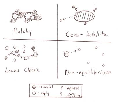
Figure
1 shows four types of metapopulations and their dispersal mechanisms from
occupied to empty habitats.
Movement among habitats is depicted with arrows. Dashed arrows depict rare
migrations. |
A
metapopulation is a group of populations (demes) connected by migrations of
individuals across populations. A
good analogy for a metapopulation is a series of towns. Towns contain their own populations and
a group of towns represent a specific metapopulation, for instance the western
suburbs. The towns are connected
and that helps facilitate movement by individuals. As some towns grow into cities from immigration and
favorable conditions, other towns decrease into villages due to emigration and
unfavorable conditions.
In
an example from nature, a series of mountain valleys may contain a
metapopulation of lilies. Lilies
may spread to new valleys through wind blown seed or flash floods. Other valleys may lose all their lilies
through herbivory, disease, stochastic events, etc. If enough suitable habitat remains and colonization of new
valleys continue, the combined populations (metapopulations) of lilies will be
stable.
Metapopulation
theory attempts to describe the movement of populations throughout suitable
habitats.
The
four models for metapopulation movement are in the figure above were developed
by Harrison in 1991.
·
Patchy – Demic system with chunks of suitable
habitat spaced relatively close together.
Individuals move freely to and from the patches, replenishing any areas
that suffer extinction (rescue effect).
Patchy metapopulations are common and extinction resistant.
·
Core-Satellite – Also called “mainland-island” or
“source-sink” because a large stable habitat supports a large stable
population. Frequent migration
occurs from the “mainland” to habitats nearby. Core-satellite is also extinction resistant.
·
Levins Classic – Populations disperse from one area to the
next. Habitats where populations
go extinct may be re-colonized or not.
Changes in the metapopulation over time is represented by the formula:
dp/dt = mp(1 – p)
– ep
p = occupied habitats.
Full occupancy p=1. Extinct p=0
m = migration rate
mp = total amount of successful dispersals
(1 – p) = unoccupied habitats
e = extinction rate
ep = total amount of patches going extinct
·
Non-equilibrium – A small patch contains the majority of the
population, because isolation or an unfavorable matrix prevents frequent
migrations. Non-equilibrium
populations are extremely vulnerable to extinction.
Fun
Fact (at least as fun as it gets) – Rodents help in environmental science
too.
Levins
developed metapopulation theory in 1970 based on the work of Soviet ecologists
concerned with rodent control during WWII. Like the Soviets, Levins was studying epidemiology
involving parasitic insects and their rodent hosts. In Levin’s model case, p represented the hosts for the parasitic insect
populations.